|
Stochastic Route Cost Minimization (SRCM™)
|
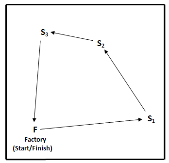
| 1) F→ S1→ S2→ S3→ F | |
| 2) F→ S1→ S3→ S2→ F | |
| 3) F→ S2→ S1→ S3→ F |
The mileage chart describing the distances between the factory and all delivery
sites is given in Table 1 below.
| F | S1 | S2 | S3 | ||
| F | 0 | 230 | 350 | 311 | |
| S1 | 230 | 0 | 290 | 360 | |
| S2 | 350 | 290 | 0 | 210 | |
| S3 | 311 | 360 | 210 | 0 |
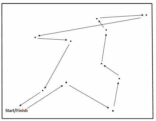
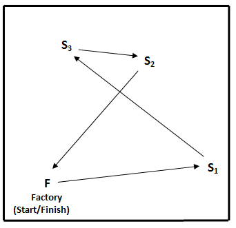
Traditional route cost minimization analysis results in the round-trip route
F→ S1→ S2→ S3→ F
(1041 miles) being the shortest round-trip mileage route as shown below in Figure 1 (map not drawn to scale):
Now let's introduce the variable of time into our search for the cheapest round-trip route. Table 2 below lists
the time taken to travel between the factory and all delivery sites. Travel times are listed in hours and decimal representations of hours
for minutes, i.e., 4.8 = 4 hours 48 minutes(60 minutes times .80 = 48.)
| F | S1 | S2 | S3 | |
| F | 0.00 | 6.00 | 4.80 | 8.90 |
| S1 | 6.00 | 0.00 | 8.80 | 4.80 |
| S2 | 4.80 | 8.80 | 0.00 | 6.00 |
| S3 | 8.90 | 4.80 | 6.00 | 0.00 |
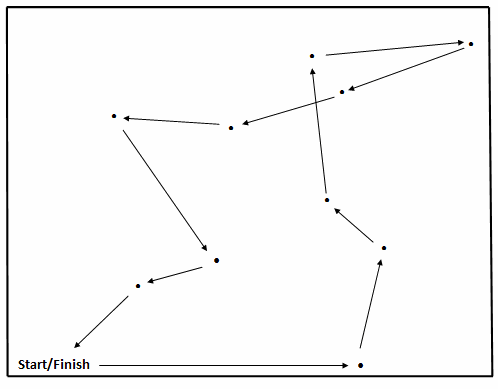
Table 2 shows that the shortest round-trip time route is F→ S1→
S3→ S2→ F (21.6 hours) as portrayed below in Figure 2:
Now let's suppose that the following cost data describes your present situation:
| Diesel fuel is $5 per gallon | |
| Delivery truck gets 8 mpg | |
| Truck driver costs $22 per hour |
Now things get interesting. To reiterate, there are only three distinct* round-trips that can be made with
one start/finish point F and three delivery points S1, S2, and S3. They are:
| 1) F→ S1→ S2→ S3→ F | |
| 2) F→ S1→ S3→ S2→ F | |
| 3) F→ S2→ S1→ S3→ F |
Table 3 below summarizes information for each trip based upon the cost data:
| Route | Time (Hours) | Distance (Miles) | Driver's Pay | Mileage Costs | Total Costs | ||
| F→ S1→ S2→ S3→ F | 29.73 | 1041 | $654 | $650 | $1,304 | ||
| F→ S1→ S3→ S2→ F | 21.57 | 1150 | $475 | $719 | $1,193 | ||
| F→ S2→ S1→ S3→ F | 27.36 | 1311 | $602 | $819 | $1,421 |
As mentioned above, the traditional approach to route cost minimization states that the shortest
round-trip in terms of miles is also the cheapest. In the present example the shortest,
and therefore the cheapest round-trip route should be F→ S1→ S2→
S3→ F at 1041 miles and a total cost of $1304. Yet Table 3 clearly shows that the round-trip
route of F→ S1→ S3→ S2→ F (1150 miles, total cost $1193), although 109 miles
longer than the shortest route, is in fact $111 cheaper! - TIME MATTERS!!!
We made the preceding example very simplistic in order to introduce you to SRCM™'s distance/time approach to route cost minimization. Unfortunately this example has a major real world flaw - we portrayed travel times as being single, constant values like the distance values. Alas, in the real world, although the travel distance of a set route rarely changes, the travel times over the same route are anything but static. Take a moment and consider the following: When someone says "the warehouse-to-Springfield run takes 4 hours", it is usually understood the travel time from the warehouse to Springfield averages 4 hours give or take, let's say, 15 minutes. This random variability in travel time is the result of the constantly changing values of a number of trip-related variables such as time of day, the driver, the weather, road construction detours, etc.
For the sake of illustration let's say the distribution of travel times to Springfield follows the well-known bell-shaped curve (a.k.a. the NORMAL DISTRIBUTION), with a mean of 240 minutes and a standard deviation of 18 minutes. Although the "distance-cost" to Springfield remains static, the "time-cost" to Springfield would fluctuate depending upon the random nature of the travel time distribution. For example, this coming Friday's delivery trip might time-cost 269 minutes, whereas next month's trip might time-cost 217 minutes.
Now let's take a fresh look at our simplistic example. When we added a static time-to-destination component
to compute travel costs the result was that the shortest route, which traditionally is the cheapest, was no
longer the cheapest route. In fact a longer mileage round-trip route was the overall cheapest. Yet, as mentioned
above, a problem with this example is that the time chart was fixed just like the distance chart. Consider now
what could happen if the travel times listed on the time chart were allowed to change randomly. Table 4 below
is a revised, more "realistic" time-to-destination presentation reflecting the random nature of travel times:
| F | S1 | S2 | S3 | |
| F | 0,0 | (6.0,.50) | (4.8,.30) | (8.9,.20) |
| S1 | (6.0,.50) | 0,0 | (8.8,.70) | (4.8,.18) |
| S2 | (4.8,.30) | (8.8,.70) | 0,0 | (6.0,.10) |
| S3 | (8.9,.20) | (4.8,.30) | (6.0,.10) | 0,0 |
The first number is the average (Mean) travel time between the two points. The next number is the Standard
Deviation of travel time between the two points, given as a percentage of an hour. Since travel times between
points can change depending on the value of the travel time variables previously mentioned, it helps to think
of the time chart as being fluid, with individual travel times between points changing randomly from time to
time, causing round-trip route costs to also become fluid. Consider the following possible scenario: let's say that the
individual travel times between points had randomly changed so that the total travel time of path
F→ S1→ S2→ S3→ F were to improve (i.e. shorten) by
approximately 17% and the round-trip travel time of path F→ S1→ S3→ S2→ F were to
worsen (i.e. lengthen) by approximately 24% then the picture would change noticeably as shown in Table 5 below:
| Route | Time (Hours) | Distance (Miles) | Driver's Pay | Mileage Costs | Total Costs | ||
| F→ S1→ S2→ S3→ F | 24.72 | 1040 | $544 | $650 | $1,194 | ||
| F→ S1→ S3→ S2→ F | 26.79 | 1150 | $589 | $719 | $1,308 | ||
| F→ S2→ S1→ S3→ F | 27.57 | 1311 | $607 | $819 | $1,426 |
Note that now the cheapest round-trip route has changed from F→ S1→ S3→ S2→ F
to F→ S1→ S2→ S3→ F! Some time later,
say two months from now, the time chart might be in a state such that the following possible configuration
Table 6 exists where the LONGEST time route is cheaper than the shortest time route. In this instance
the cheapest path has the longest time and shortest distance, whereas the cheapest route in Table 5 had
the shortest route time and the shortest distance.
| Route | Time (Hours) | Distance (Miles) | Driver's Pay | Mileage Costs | Total Costs | ||
| F→ S1→ S2→ S3→ F | 29.00 | 1040 | $650 | $650 | $1,288 | ||
| F→ S1→ S3→ S2→ F | 27.00 | 1150 | $719 | $719 | $1,313 | ||
| F→ S2→ S1→ S3→ F | 25.93 | 1311 | $819 | $819 | $1,390 |
Granted, the time difference in this very simple example is only 2 hours with a savings of a measly $25.
Still, being able to free a driver 2 hours earlier than before could very well be worth a great deal more
than just saving $25. Whatever the case, hopefully the point has been made: the overall cheapest round-trip
route changes from time to time.
In a previous paragraph we mentioned that "a more realistic route with 10 delivery points generates 1,814,400 distinct round-trip routes - and only one of these is the cheapest!". That cheapest referred to shortest distance. Now that we have demonstrated how fluctuating travel times effect costs, adding the "time variable" into the search for a cheapest route makes the number of possible round-trip routes immense. Making the situation even more complex is the fact that in the real world, travel times can be quite different from the "well-behaved" normal curve. The travel times might follow more "exotic" distributions such as POISSON, LOGNORMAL, GAMMA, etc.
It might just be that the warehouse-to-Springfield run can take anywhere from 50 to 75 minutes depending on the random value of trip-time variables. Furthermore this time interval could in fact show, depending on the value of the variables, a kind of random "lopsidedness" so that the concept of "average" travel time becomes meaningless. For example, let's say that at the moment the values of the variables are such that ROUGHLY 70% of the time the Springfield trip takes about 60 minutes, give or take 10 minutes and roughly 30% of the time it takes 75, give or take 15 minutes.
The enormity of the problem of finding the cheapest round-trip route should be quite clear - at any particular point in time there exists a single, cheapest route from among a truly astronomical number of possible round-trip routes. Yet this cheapest route will most likely change in the near future and no longer be the cheapest route. Maybe it will take a month, or even a year - but it will change, and sometimes dramatically.
Now obviously you can't keep changing routes every time a better one comes along, it would be a logistical
nightmare! No, the answer is to implement SRCM™ which has the ability to take into account the random,
probabilistic variations of future travel times when searching for the most cost effective, "longest lasting" round-trip delivery route.
The simple answer is: "Seeing is believing". The great advantage of our SRCM™ service
is that you can see that the minimal cost route we provide for you is indeed minimal - all you have to do
is plug in your own data and see that we have saved you money. It's right there in front of your eyes - no waiting
to see if our new route will save you money, you can immediately see that it does.
* We consider route S0→S1→S2→S3→S0
to be non-distinct from route S0→S3→S2→S1→S0
top
back